Chapter 10 4) Run Random Forest
Computationally, a subset of the training dataset is generated by bootstrapping (i.e. random sampling with replacement). For each subset a decision tree is grown and, at each split, the algorithm randomly selects a number of variables (mtry) and it computes the Gini index to identify the best one. The process stops when each node contains less than a fixed number of data points. The fundamental hyperparameters that needs to be defined in RF are mtry and the total number of trees (ntrees).
The prediction error on the training dataset is finally assessed by evaluating predictions on those observations that were not used in the subset, defined as “out-of-bag” (OOB). This values is used the optimize the values of the hyperparameters, by a trial and error process (that is, trying to minimize the OOB estimate of error rate).
# Set the seed of R‘s random number generator,
## this is useful for creating simulations that can be reproduced.
set.seed(123)

# Run RF model
RF_LS<-randomForest(y=LS_train$LS, x=LS_train[1:8],data=LS_train, ntree=500, mtry=3,importance=TRUE)
10.1 4.1) RF main outputs
Printing the results of RF allows you to gain insight into the outputs of the implemented model, namely the following: - a summary of the model hyperparameters - the OOB estimate of error rate - the confusion matrix; in this case a 2x2 matrix used for evaluating the performance of the classification model (1-presence vs 0-absence).
The plotting the of the error rate is useful to estimate the decreasing values on the OOB and on the predictions (presence (1) / absence (0)) over increasing number of trees.
##
## Call:
##  randomForest(x = LS_train[1:8], y = LS_train$LS, ntree = 500,      mtry = 3, importance = TRUE, data = LS_train)
##                Type of random forest: classification
##                      Number of trees: 500
## No. of variables tried at each split: 3
##
##         OOB estimate of  error rate: 16%
## Confusion matrix:
##      0    1 class.error
## 0 1691  397   0.1901341
## 1  267 1795   0.1294859
# Show the predicted probability values
RF.predict <- predict(RF_LS,type="prob")
head(RF.predict) # 0 = absence ; 1 = presence## 0 1
## 2063 0.28795812 0.71204188
## 1750 0.02259887 0.97740113
## 688 0.76506024 0.23493976
## 3301 1.00000000 0.00000000
## 4401 0.98514851 0.01485149
## 1166 0.05113636 0.94886364# Plot the OOB error rate
plot(RF_LS)
legend(x="topright", legend=c("perd 0", "pred 1", "OOB error"),
col=c("red", "green", "black"), lty=1:2, cex=0.8)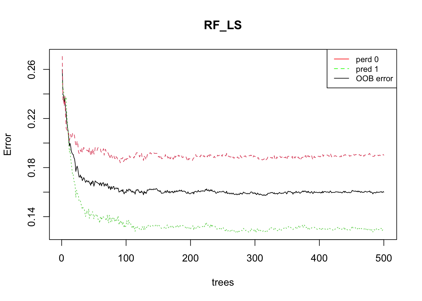
10.2 4.2) Model evaluation
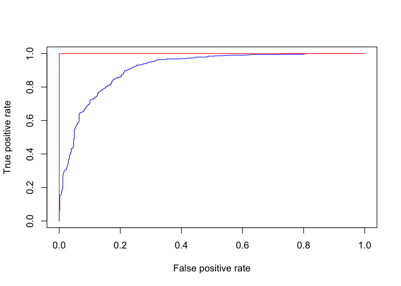
The prediction capability of the implemented RF model can be evaluated by predicting the results over previously unseen data, that is the testing dataset. The Area Under the “Receiver Operating Characteristic (ROC)” Curve (AUC) represents the evaluation score used here as indicator of the goodness of the model in classifying areas more susceptible to landslides. ROC curve is a graphical technique based on the plot of the percentage of correct classification (the true positives rate) against the false positives rate (occurring when an outcome is incorrectly predicted as belonging to the class “1” when it actually belongs to the class “0”), evaluates for many thresholds. The AUC value lies between 0.5, denoting a bad classifier, and 1, denoting an excellent classifier, which, on the other hand, can in this case overfit.
# Make predictions on the testing dataset
RFpred_test <- predict(object = RF_LS, newdata = LS_test, type="prob")

# Make predictions on the validation dataset (taining using the Out-of-bag)
RFpred_oob <- predict(object = RF_LS, newdata = LS_train, type="prob", OOB=TRUE)

roc_test <- roc(LS_test$LS, RFpred_test[,2])
roc_oob <- roc(LS_train$LS, RFpred_oob[,2])

plot.new()
plot(1-roc_test$specificities, roc_test$sensitivities, type = 'l', col = 'blue',  xlab = "False positive rate", ylab = "True positive rate")
lines(1-roc_oob$specificities, roc_oob$sensitivities, type = 'l', col = 'red')