Chapter 3 2) Plotting vector dataset
The spatial component of geodata uses geometric primitives like point, line, and polygon to represent the single features. Each feature in a geodataset is associated with various attributes providing detailed quantitatives and qualitatives information. A single geodataset includes features of the same type, represented by using the same class of primitive.
The three basic geometric vector primitives have the following characteristics:
- Points: defined by a single pair of coordinates (x, y) representing a specific location. Used to represent small objects like weather stations, city center, or to identify single features in a geohazard inventory (e.g., earthquake’s epicenter, landslides location, wildfires, etc.).
- Lines: defined by pairs of coordinates connected to each other, representing linear features such as roads or rivers network, pathways, railway, etc.
- Polygons: defined by a series of connected coordinates that enclose an area, representing features such as lakes, administrative units, vegetation patches, burned area, landslides footprint, etc.
3.1 2.1) Load libraries and vector dataset
The package sf (Pebesma 2022) has been designed to work with vector datasets as “simple features” in R. Each feature is represented by one row in the data frame, with attributes stored as columns and spatial information stored in a special geometry column.
As a toy example, we will work with the geodataset of administrative boundaries in the Canton of Vaud (Switzerland). This dataset is available in shapefile format, one of the most widely used file formats for vector geospatial data.
A shapefile include multiple files allowing to store different kind of object:
*shp: features’ geometries (i.e., the geometric vector primitive used to describe the feautues).
*dbf: the attribute describing the characteristics of the features (i.e., tabular information).
*shx: shape index format, an index file for the geometry data.
*prj: storing the coordinate reference systems, defining how the geometries are projected on the Earth’s surface.
To read a shapefile, you only need to specify the filename with “.shp” extension. However, it is important to have all related files in the same directory. Having all these files ensures that the shapefile is read correctly and all necessary information is available for analysis.
Shapefiles are imported and converted as sf objects using the command st_read(). By setting the argument “quiet = FALSE” suppresses the output from the console when importing geodata.
## Reading layer `Canton_de_Vaud' from data source
##   `/Users/hliu5/Documents/AGDAbook/data/RGIS/Canton_de_Vaud.shp'
##   using driver `ESRI Shapefile'
## Simple feature collection with 315 features and 4 fields
## Geometry type: POLYGON
## Dimension:     XY
## Bounding box:  xmin: 2494306 ymin: 1115149 xmax: 2585462 ymax: 1203493
## Projected CRS: CH1903+ / LV95
3.2 2.2) Plot vector features
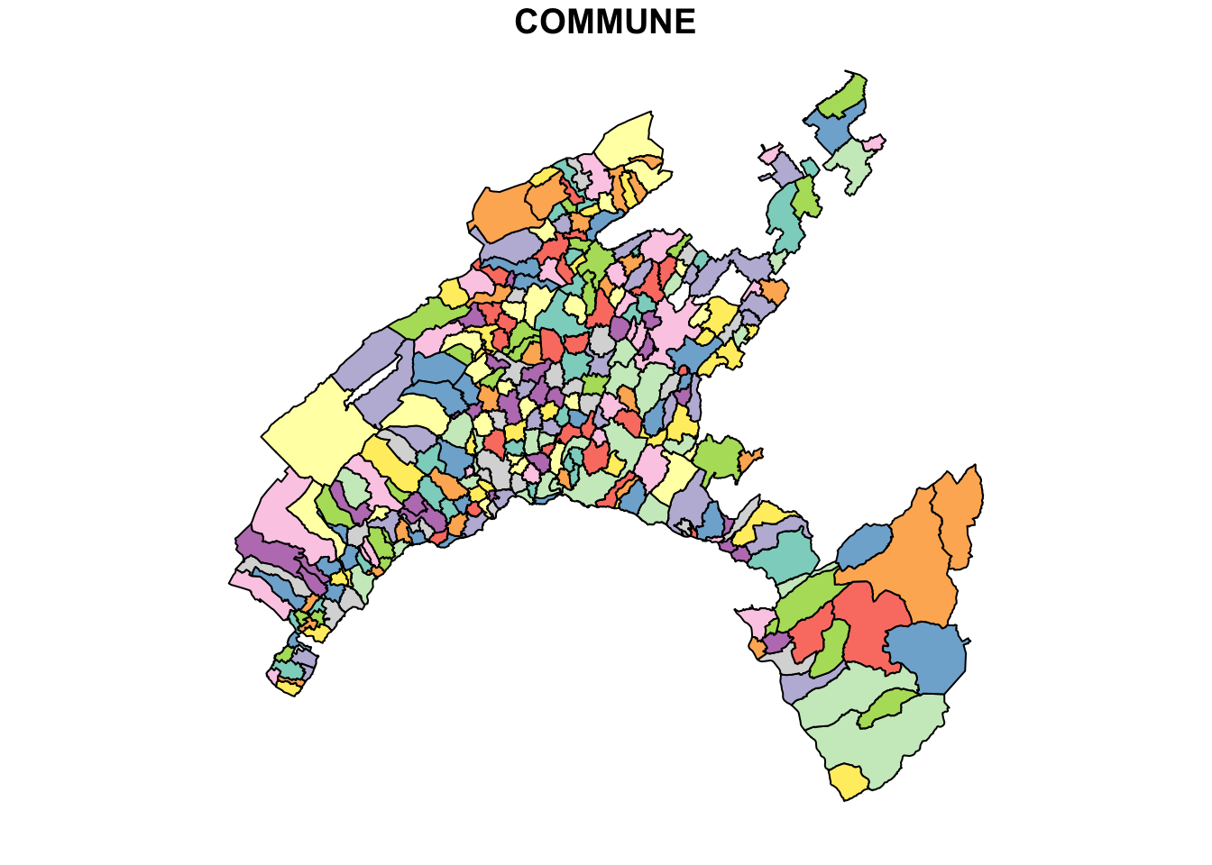
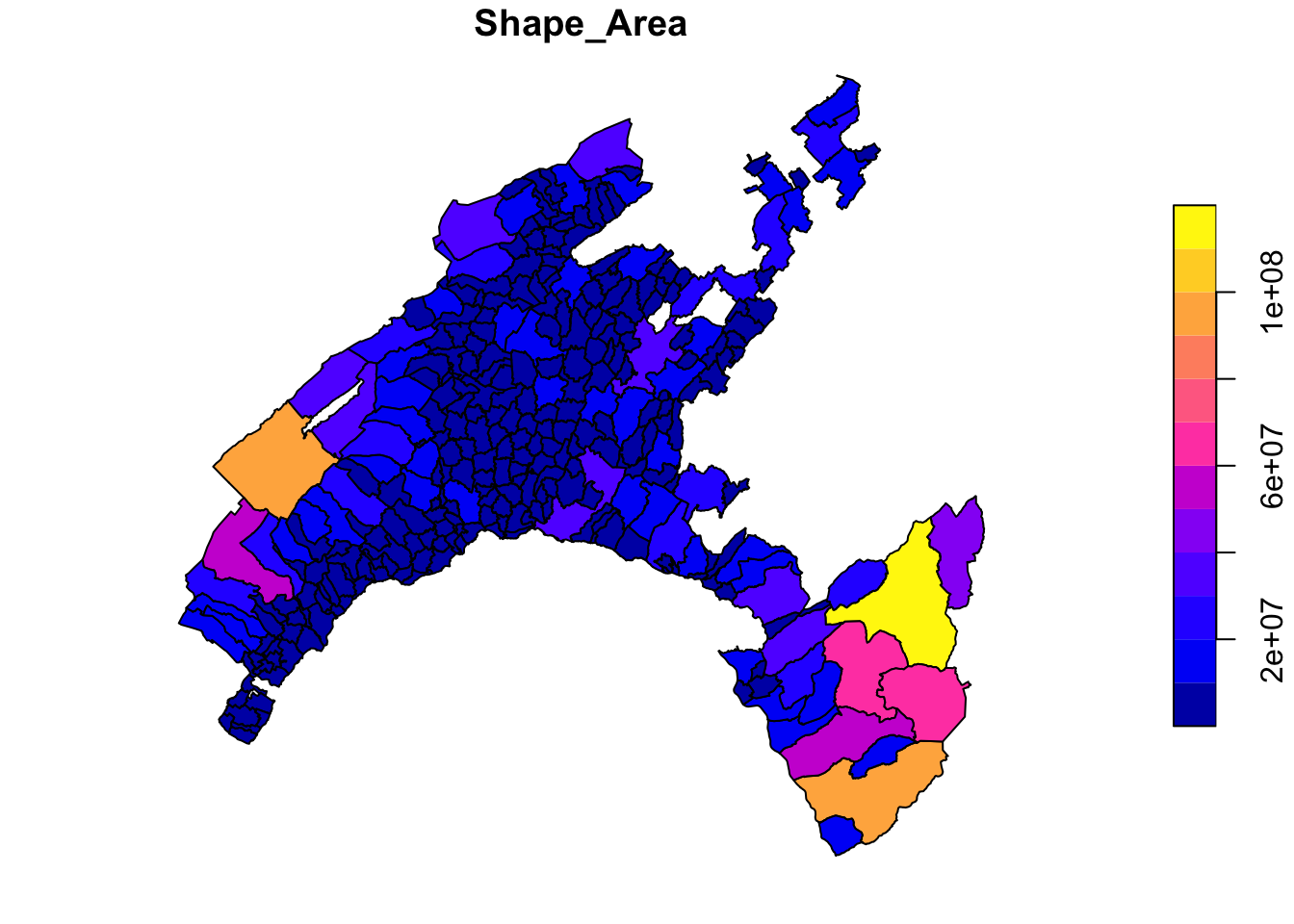
Basic maps are created in sf with the command plot(). By default this creates a multi-panel plot: one plot for each variable included in the geodata (i.e., each column).
This command can be followed by the name variable that you wish to display.
## Classes 'sf' and 'data.frame':   315 obs. of  5 variables:
##  $ COMMUNE   : chr  "Payerne" "Rossinière" "Vallorbe" "Puidoux" ...
##  $ NUMERO_COM: num  5822 5842 5764 5607 5745 ...
##  $ Shape_Leng: num  30547 21405 27147 31111 28268 ...
##  $ Shape_Area: num  24178457 23354685 23190781 22858943 22501915 ...
##  $ geometry  :sfc_POLYGON of length 315; first list element: List of 1
##   ..$ : num [1:783, 1:2] 2559434 2559258 2559286 2559263 2559337 ...
##   ..- attr(*, "class")= chr [1:3] "XY" "POLYGON" "sfg"
##  - attr(*, "sf_column")= chr "geometry"
##  - attr(*, "agr")= Factor w/ 3 levels "constant","aggregate",..: NA NA NA NA
##   ..- attr(*, "names")= chr [1:4] "COMMUNE" "NUMERO_COM" "Shape_Leng" "Shape_Area"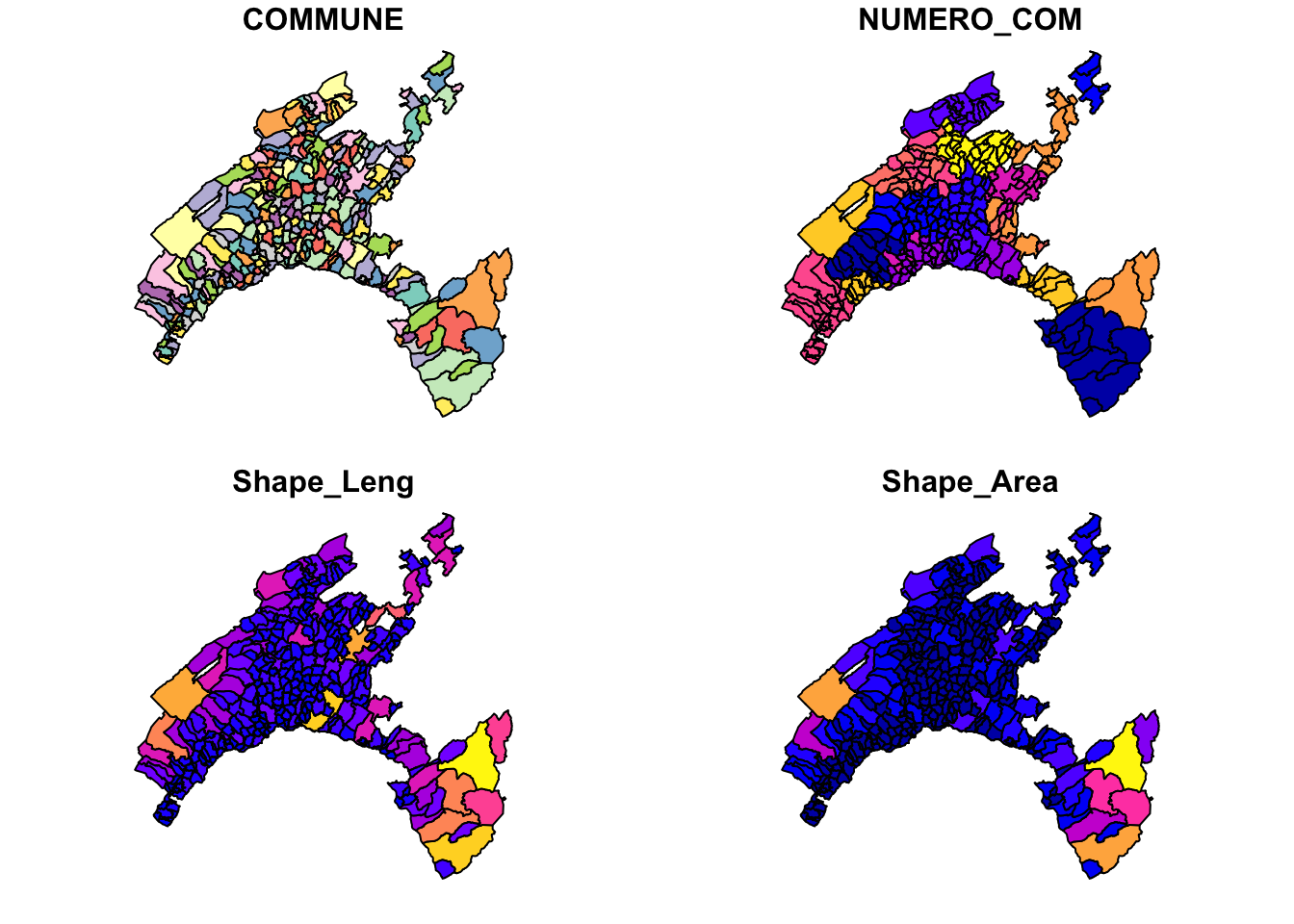
A legend with a continuous color scale is produced by default if the object to be plotted belong is numeric.
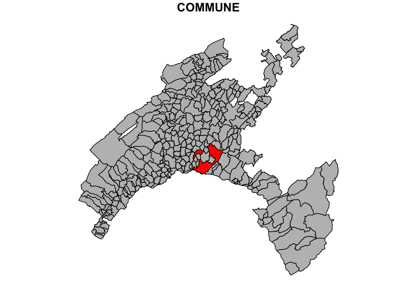
Different operations can be performed to customize the map. For instance, it should be great to set up the municipality of Lausanne as the specially red to show the geographic correspondence.
# Extract the Lausanne boundary
Vaud_Lausanne = vaud[vaud$COMMUNE == "Lausanne", ]

# Union and merge the geometry
Lausanne = st_union(Vaud_Lausanne)

# plot the Lausanne municipality over a map of Canton of Vaud
plot(vaud["Shape_Area"], reset = FALSE)
plot(Lausanne, add = TRUE, col = "red")