Chapter 4 3) Plotting raster dataset
Raster data are different from vector data in that they are referenced to a regular grid of rectangular (usually square) cells, called pixels.
The spatial characteristics of a raster dataset are defined by its spatial resolution (the height and width of each cell) and its origin (typically the upper left corner of the raster grid, which is associated with a location in a coordinate reference system).
Raster data is highly effective for modeling and visualizing continuous spatial phenomena such as elevation, temperature, and precipitation. Each cell in the grid captures a value representing the attribute at that specific location, allowing for smooth and detailed gradients across the study area. This format is also effective in representing categorical variables such as land cover, where each cell is associated with a class value.
Common raster formats used used for spatial analses include:
GeoTIFF (.tif, .tiff):
- A widely used format that includes geographic metadata such as coordinates and projection information, making it easy to integrate with GIS applications.
ESRI Grid:
- A proprietary format developed by ESRI for use with its software, such as ArcGIS. It supports both integer and floating-point grids.
Erdas Imagine (.img):
- A format developed by ERDAS for its Imagine software, often used for remote sensing data and satellite imagery. It supports large files and multiple bands.
NetCDF (.nc):
- Stands for Network Common Data Form, used for array-oriented scientific data, including GIS data. It supports multidimensional data arrays, making it suitable for complex environmental and atmospheric data.
HDF (Hierarchical Data Format):
- Similar to NetCDF, HDF is used for managing and storing large amounts of data, especially in scientific computing. It supports various data types and is used for satellite imagery and climate data.
ASCII Grid (.asc):
- A simple, text-based raster format where each cell value is represented by a number in a grid layout. It’s easy to read and edit with a text editor.
These formats vary in terms of compression, metadata support, and suitability for different types of raster data, from simple images to complex scientific datasets.
4.1 3.2) Load libraries and raster dataset
The terra package provides a variety of specialized classes and functions for importing, processing, analyzing, and visualizing raster datasets (Hijmans 2022). It is intended to replace the raster package, which has similar data objects and the function syntax as terra package. However, the terra package contains several major improvements, including faster processing speed for large raster.
## Warning: package 'terra' was built under R version 4.3.3## terra 1.7.78##
## Attaching package: 'dplyr'## The following objects are masked from 'package:terra':
##
## intersect, union## The following objects are masked from 'package:stats':
##
## filter, lag## The following objects are masked from 'package:base':
##
## intersect, setdiff, setequal, union# Load the libraries
library(terra)
# Load the raster data
Vaud_dem <- rast("data/RGIS/DEM.tif")
# Inspect the raster
Vaud_dem## class : SpatRaster
## dimensions : 3524, 3647, 1 (nrow, ncol, nlyr)
## resolution : 25, 25 (x, y)
## extent : 494300, 585475, 115150, 203250 (xmin, xmax, ymin, ymax)
## coord. ref. : CH1903 / LV03 (EPSG:21781)
## source : DEM.tif
## name : DEM
## min value : 372.0
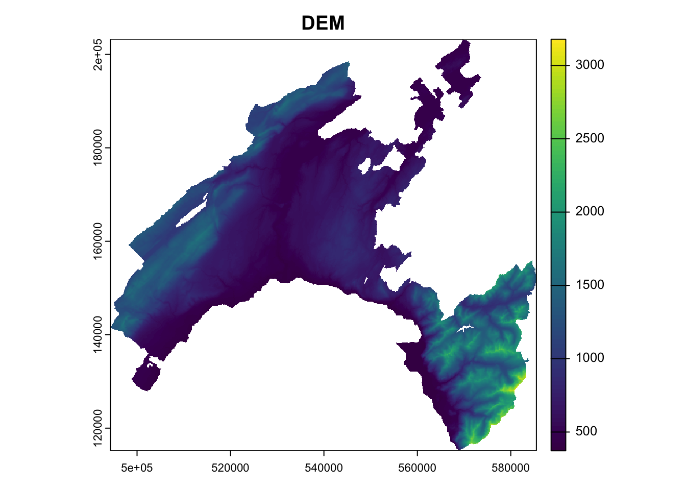
## max value : 3200.14.2 3.2) Plot raster features
Raster objects can be imported using the function rast() and exported using writeRaster(), specifing the format argument.
As a toy example, we will work with the raster *.tif representing the digital elevation model (DEM) of Canton Vaud.
Similar to the sf package for ploting vector data, terra also provides plot() methods for its own classes.