Chapter 9 2) Import and process geodata
Import landslides punctual dataset presences and absences (LS_pa) and predictors (in raster format). This help the exploratory data analyses step and to understand the input data structure.
9.1 2.1) Landslides dataset
The landslide inventory has been provided by the environmental office of the canton of Vaud. Only shallow landslides are used for susceptibility modelling. One pixel per landslide-area (namely the one located at the highest elevation) has been extracted. Since the landslide scarp is located in the upper part of the polygon, it makes sense to consider the highest pixel to characterize each single event.
Our model includes the implementation of the landslide pseudo-absences, which are the areas where the hazardous events did not took place (i.e. landslide location is known and the mapped footprint areas are available, but the non-landslide areas have to be defined). Indeed, to assure a good generalization of the model and to avoid the overestimation of the absence, pseudo-absences need to be generated in all the cases where they are not explicitly expressed. In this case study, an equal number of point as for presences has been randomly generated in the study area, except within landslides polygons, lakes and glaciers (that is what is called “validity domain”, where events could potentially occur).
The landslides dataset
# Import the boundary of Canton Vaud
Vaud <- vect("data/RF/Vaud_CH.shp")
Lake <- vect("data/RF/Lakes_VD.shp")


# Import the landslides dataset (dependent variable)
LS_pa <- read.csv("data/RF/LS_pa.csv")

# Convert the numeric values (0/1) as factor
##(i.e. categorical value)
LS_pa$LS<-as.factor(LS_pa$LS)

LS_vect<-vect(LS_pa, geom=c("X", "Y"),crs=crs(Vaud))

# Display the structure (str) and result summaries (summary)
str(LS_vect)
summary(LS_vect)

# Plot the events
plot(Vaud)
plot(Lake, col="lightblue", add=TRUE)
plot(LS_vect, col=LS_pa$LS, pch=20, cex=0.5, add=TRUE)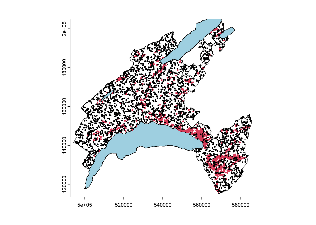
9.2 2.2) Predictor variables
Selecting predictive variables is a key stage of landslide susceptibility modelling when using a data-driven approach. There is no consensus about the number of variables and which variables should be used. In the present exercice e will use the following:
DEM (digital elevation model): provided by the Swiss Federal Offce of Topography. The elevation is not a direct conditioning factor for landslide; however, it can reflect differences in vegetation characteristics and soil
Slope: is one of the most explicating factor in landslide susceptibility modelling.
\[Slope = arctan(\sqrt{(dz/dx)^2 + (dz/dy)^2)} * (\pi/2)\]
Curvature: curvature is widely used in landslide susceptibility modelling. It allows assessing the water flow acceleration and sediment transport process (profile curvature) and the water flow propensity to converge and diverge (plan curvature). They were derived from DEM using the curvature tool in ArcGIS.
TWI (topographical water index): topography plays a key role in the spatial distribution of soil hydrological conditions. Defining \(\alpha\) as the upslope contributing area describing the propensity of a cell to receive water, and \(\beta\) as the slope angle, TWI (compute by the formula below), reflects the propensity of a cell to evacuate water:
\[TWI=ln(\alpha/tan(\beta))\]
Distance to roads: roads build in mountainous areas often cut the slope, weakening the cohesion of the soil. Moreover, roads surfaces are highly impermeable. This raster has been elaborated using the euclidean distance tool in ArcGIS, from the swissTLMRegio map where roads are represented by lines.
Land Cover: developed by the Swiss administration and based on aerial photographs and control points. It includes 27 categories distributed in the following 6 domains: human modified surfaces, herbaceous vegetation, shrubs vegetation, tree vegetation, surfaces without vegetation, water surfaces (glaciers included).
Geology: The use of the lithology increase the performance of the susceptibility landslide models. We use here the map elaborated by the Canton Vaud, defining the geotypes and reclassified in 10 classes in order to differentiate sedimentary rocks.
Than the predictor variables have to be aggregated into single object, storing multiple raster. We use here the generic function c to combine the single raster into multiple raster objet.
## Import raster (independent variables) 25 meter resolution

landCover<-as.factor(rast("data/RF/landCover.tif"))
geology<-as.factor(rast("data/RF/Geological_classes.tif"))

planCurv<-rast("data/RF/plan_curvature.tif")/100
profCurv<-rast("data/RF/profil_curvature.tif")/100

# this because ArcGIS multiply curvature values by 100

TWI <- rast("data/RF/TWI.tif")
Slope <- rast("data/RF/Slope.tif")
dem <- rast("data/RF/DEM.tif")
dist <- rast("data/RF/dist_roads.tif")

# Combine raster

features<-c(dist, dem, landCover, TWI, planCurv, profCurv, Slope, geology)

# renames features as in LS
names(features)<-c("distRoad", "DEM", "landCover", "TWI", "planCurv", "profCurv", "slope", "geology")

# mask to DEM extension
features <- terra::mask(features, dem)

plot(features)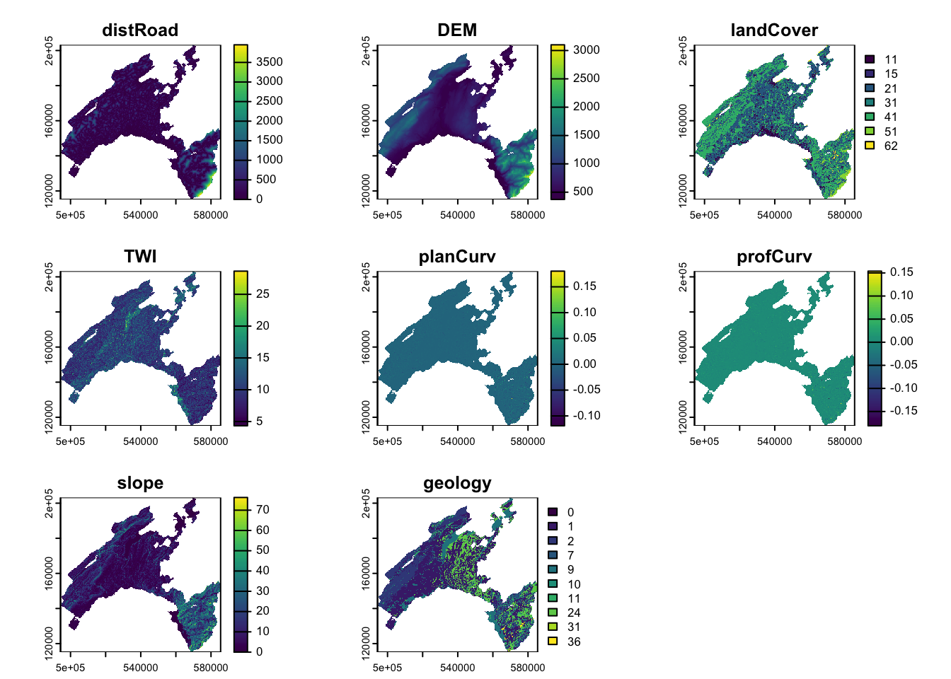
9.2.1 2.2.1) The use of categorical variables in Machine Learning
The majority of ML algorithms (e.g., support vector machines, artificial neural network, deep learning) makes predictions on the base of the proximity between the values of the predictors, computed in terms of euclidean distance. This means that these algorithms can not handle directly categorical values (i.e., qualitative descriptors). Thus, in most of the cases, categorical variables need to be transformed into a numerical format. One of the advantage of using Random Forest (as implemented in R) is that it can handle directly categorical variables, since the algorithm operate by constructing a multitude of decision trees at training time and the best split is chosen just by counting the proportion of each class observation.
To understand the characteristics of the categorical variables, you can plot the tow raster Land Cover and Geology by using their original classes and look at the attribute table to analyse the corresponding definitions.
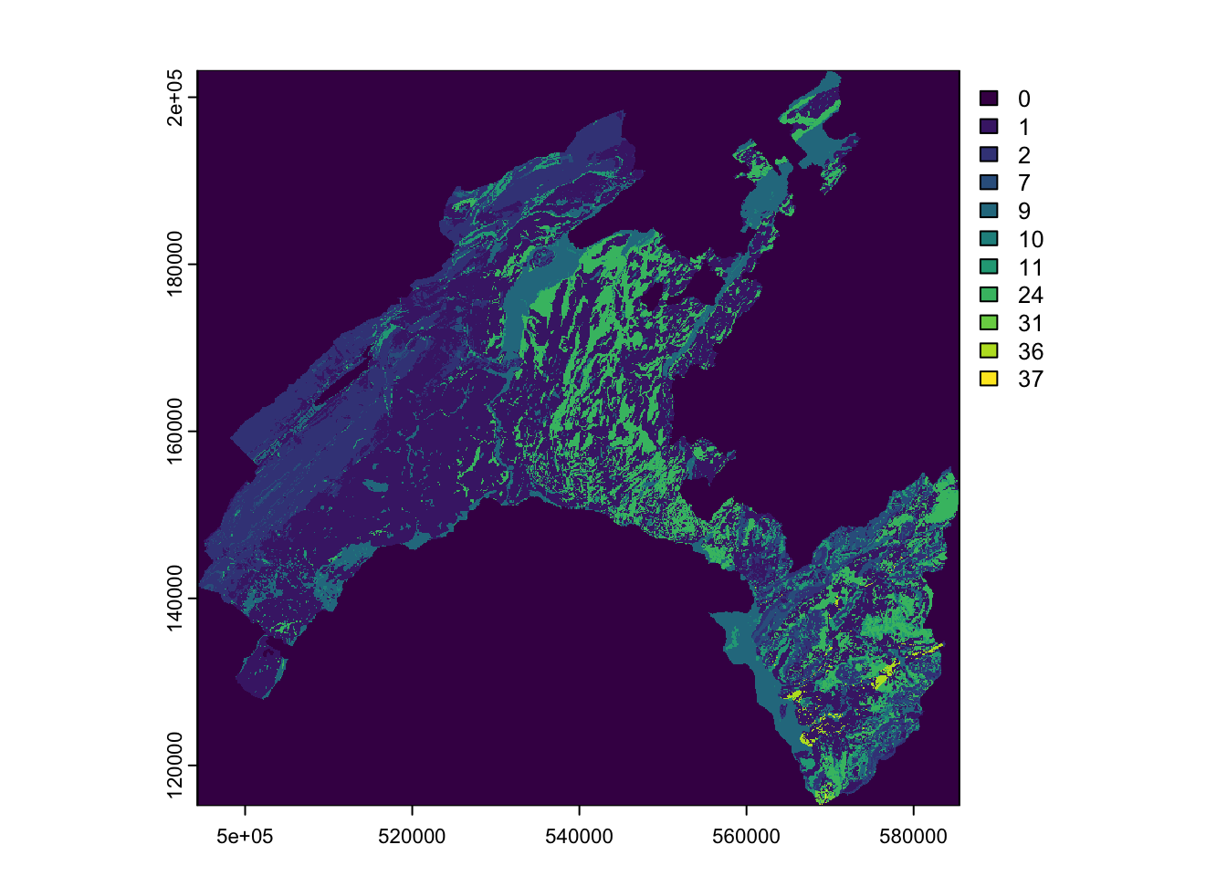
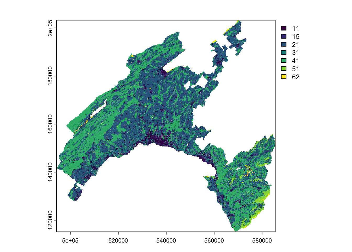
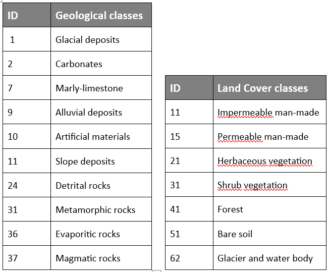
(#fig:cat_class)Categorical variables
9.3 2.3) Extract velues
In this step, you will extract the values of the predictors at each location in the landslides (presences and absences) dataset. The final output represents the input dataset with dependent (LS = landslides) and independent (raster features) variables.
The final input dataset
# Extract values from the raster dataset (features)
LS_input <-extract(features, LS_vect, method="simple",  xy=TRUE)

LS_input$LS <- as.factor(LS_vect$LS) # add LS
str(LS_input) # explore the dataset

# remove extra column (ID)
LS_input <- LS_input[,2:ncol(LS_input)]
LS_input<-na.omit(LS_input)

# Explore the newly created input dataset
head(LS_input)
str(LS_input)
9.3.1 2.3.1) Split the input dataset into training (80%) and testing (20%)
A well-established procedure in ML is to split the input dataset into training, validation, and testing.
The training dataset is needed to calibrate the parameters of the model, which will be used to get predictions on new data.
The purpose of the validation dataset is to optimize the hyperparameter of the model (training phase). NB: in Random Forest this subset is represented by the Out-Of-Bag (OOB)!
To provide an unbiased evaluation of the final model and to assess its performance, results are then predicted over unused observations (prediction phase), defined as the testing dataset.
# Shuffle the rows
set.seed(123) # to ensure reproducibility
LS_input_sh<-LS_input [sample(nrow(LS_input), nrow(LS_input)), ]

# Split the input dataset into training (80%) and testing (20%)
n <- nrow (LS_input_sh)
set.seed(123)
n_train <- round(0.80 * n)
train_indices <- sample(1:n, n_train)

# Create indices
LS_train <- LS_input_sh[train_indices, ]
LS_test <- LS_input_sh[-train_indices, ]

# Count the number of elements in the two subset: training and testing
count(LS_train)
count(LS_test)